flempar_parliamentary work

knitr::opts_chunk$set(echo = TRUE)

In this post we delve into the get_work() function and the parameters you can specify to query for more specific information.

Example 1 - Basic functionalities

First, we will query for all debates on current affairs (one possible type of parliamentary work - and the default option) organized in January-August 2022. We use the get_work() function. Indeed, in contrast to the get_mp function, you always need to specify a date range using the following arguments:

• date_range_from: the start date YYYY-MM-DD
• date_range_to: the end date YYYY-MM-DD

work_b <- get_work(date_range_from="2022-01-01"
                    , date_range_to="2022-08-31")

work_b %>%
  tibble() %>%
  head(10) %>% View

As an enormous amount of data can be retrieved through the get_work() function, it is highly recommended to test your query on a limited date range before expanding the date range to comprise multiple months to years.

Note also that we include a chunk of code that lets you inspect the first 10 observations in the data frame created. This allows you to get a feel of the data obtained before diving in deeper. This is how the resulting data frame looks like:

Inspecting this data frame, shows you what the default parameters deliver. Namely, the “details” about “debates” in current affairs in “plenary” sessions for the “dates” specified. Though, much more is possible!

The get_work() function has the following arguments:

• date_range_from: the start date YYYY-MM-DD
• date_range_to: the end date YYYY-MM-DD
• fact: options include “written_questions”, “debates”, “oral_questions_and_interpellations”, “parliamentary_initiatives”, and “council_hearings”
• type: options include “details”, “speech” and “documents”
• plen_comm: choose between plenary “plen” and commission “comm” sessions
• use_parallel: Boolean of which the default value is set to TRUE, select FALSE in case you do not have multiple workers to speed up the calls made
• raw: Boolean of which the default value is set to FALSE, select TRUE in case you wish to retrieve the unprocessed data
• extra_via_fact: Boolean of which the default value is set to FALSE, select TRUE in case you wish to retrieve the unique identifiers of documents outside the date range specified but linked to the “fact”.

So let’s, for instance, query for some specific type of parliamentary work conducted in 2021. Here, we opt to retrieve data about parliamentary initiatives (fact="parliamentary_initiatives") discussed in the plenary (plen_comm="plen") sessions (date_range_from="2021-01-01"and date_range_to="2021-12-31"). We also specify that we are interested in the type="details" as this will deliver us a data frame containing the essentials about each parliamentary initiative.

pi_work <- get_work(date_range_from="2021-01-01"
                    , date_range_to="2021-12-31"
                    , fact="parliamentary_initiatives"
                    , type="details"
                    , plen_comm="plen")

pi_work %>%
  tibble() %>%
  head(10) %>% View

Now we can inspect the data a bit more. Something you can check, for example, is which topics are covered in the parliamentary initiatives at that time. We use some dplyr code, in this case count() to quickly count the unique values in the column result_thema_1.

pi_work %>% count(result_thema_1, sort = T) -> work_topics
work_topics

Example 2 - Retrieving documents related to parliamentary work

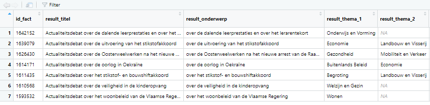
Here, we opt to retrieve data about written questions (fact="written questions") issued in March 2022 (date_range_from="2022-03-01"and date_range_to="2022-03-31"). Importantly, we specify that we are interested in type="document" as this will deliver us a data frame containing the documents related to each written question in the selection.

wq_work_doc <- get_work(date_range_from="2022-03-01"
                    , date_range_to="2022-03-31"
                    , fact="written_questions"
                    , type="document")  

wq_work_doc %>%
  tibble::tibble() %>%
  head(10) %>% View

This call delivers you a data frame with (at least) the following columns:

• id_fact: unique identifier linking to the specific parliamentary activity the document is associated with (in this example, the written question)
• text: each row in this column contains the text contained in the document

The data frame can be manipulated further to make it ready for text analysis. First, matching the data frame with the details of its associated written questions is possible via id_fact.

wq_work <- get_work(date_range_from="2022-03-01"
                    , date_range_to="2022-03-31"
                    , fact="written_questions"
                    , type="details")  

wq_docs_details <- left_join(wq_work, wq_work_doc, by=c("id_fact")) 

Another element here is that we can search these documents for specific key words occurring in one of them. For this, we use the search_terms() function with the following arguments:

• text_field: fill in the column name of the text field in c(“XXX”), multiple columns can be specified at once as c(“XXX”, “XXX”, …)
• search_terms: fill in the term(s) you want the documents checked for

Here, we opt to retrieve data about the PFOS/PFAS debate in Belgium (search_terms = c("PFOS", "PFAS")).

wq_docs_details %>%
  as_tibble() %>%
  search_terms(text_field = c("text"), search_terms = c("PFOS", "PFAS")) -> PFOS

Note that to get a good feel of the data, it is often recommended to sort the data frame by id_fact (e.g. when retrieving documents about fact="parliamentary_initiatives, multiple documents are associated to one initiative). This thus gives you a clearer overview of all documents related to one unique ‘activity’.

Example 3 - Retrieving speech related to parliamentary work

For this example, we opt to retrieve data about oral questions and interpellations (fact="oral_questions_and_interpellations") discussed in the committee meetings (plen_comm="comm") of March 2022 (date_range_from="2022-03-01"and date_range_to="2022-03-31"). Next, we specify that we are interested in the type="speech" as this will deliver us a data frame containing the ‘speech’ or spoken word by MPs and ministers related to each oral question in the selection.

oq_speech <- get_work(date_range_from="2022-03-01"
                    , date_range_to="2022-03-31"
                    , fact="oral_questions_and_interpellations"
                    , type="speech"
                    , plen_comm="comm") 

This call delivers you a data frame with the following columns:

• journaallijn_id: the unique identifier for each action-reaction sequence related to the same oral question.
• text: each row in this column contains the ‘speech’ per individual speaker.
• sprekertitel: identifies who is speaking.
• persoon_id: the unique identifier for each individual.

Matching this data frame with the details of these oral questions is possible via the journaallijn_id. Here, we show you how to extract the journaallijn_id from the details data frame through unnesting the column result_procedureverloop and then the column journaallijn.

oq_details <- get_work(date_range_from="2022-03-01"
                    , date_range_to="2022-03-31"
                    , fact="oral_questions_and_interpellations"
                    , type="details"
                    , plen_comm="comm"
                    , use_parallel=TRUE) 

oq_details %>% 
  unnest(result_procedureverloop) %>% 
  unnest_wider(journaallijn, names_sep = "_") -> oq_details_jln

Upon inspection of this data frame, you will notice that the journaallijn_id is not automatically filled in across all rows. To end up again with non-repeated observations (i.e. unique rows), we filter out those rows not containing the journaallijn_id.

oq_details_jln %>%
  filter(!is.na(journaallijn_id)) -> oral_questions

Now we are ready to join the oral_questionsdata frame with the mp_oq_speech data frame containing the ‘speech’ per oral question.

oq_speech %>% 
  mutate(journaallijn_id = as.numeric(journaallijn_id)) -> oq_speech

questions_speech <- left_join(oral_questions, oq_speech, by=c("journaallijn_id")) 

Finally, we can also search these spoken words for specific key words occurring. We again use the search_terms() function. We opt to retrieve data about the PFOS/PFAS debate in Belgium (search_terms = c("PFOS", "PFAS")).

questions_speech %>%
  as_tibble() %>%
  search_terms(text_field = c("text"), search_terms = c("PFOS", "PFAS")) -> PFAS_oq

Example 4 - ADVANCED: Extra unnesting of lists

Though, as you may have noticed from your first inspection of the data frame, the get_work() function from the get-go confronts you with a couple of nested columns. We will go over several examples to dig up relevant information from these lists in lists. Keep in mind that it is recommended to go step-by-step when going deeper into the lists as it is far too easy to end up with a giant unfitting data frame when combining multiple ‘unnestings’ at once without knowing the exact content of the data stored within the lists.

1. Topics by type of activity: unnesting of the column result_objecttype

Here, we use the pi_work data frame that we created in the first example of this post to demonstrate how to ‘unnest’ columns.

pi_work %>%
  select(id_fact, result_objecttype, result_thema_1) %>%
  unnest_wider(result_objecttype) %>%
  select(id_fact, naam, result_thema_1) -> work_type_topics
work_type_topics

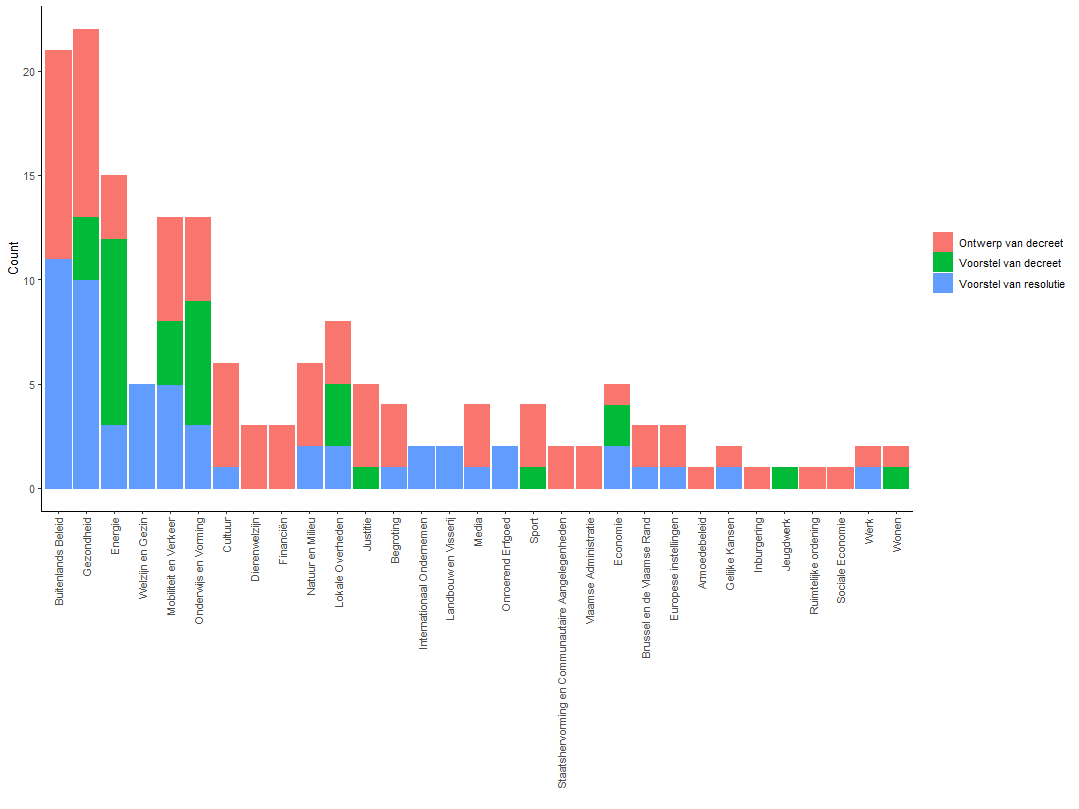
Now we can make a count of the observations by relevant types of activity or visualize the results.

work_type_topics %>%
  filter(naam == "Ontwerp van decreet" 
         | naam == "Voorstel van decreet" 
         | naam == "Voorstel van resolutie") -> work_type_topics
work_type_topics

work_type_topics %>% 
  group_by(naam) %>%
  count(result_thema_1, sort = T) -> work_type_topics_c
work_type_topics_c

plot5 <- ggplot(work_type_topics_c, aes(x = reorder(result_thema_1, -n), y = n, fill= naam, colour = naam)) + 
  geom_bar(stat = "identity") +
  labs(x="", y = "Count") + 
  theme_classic() +
  theme(axis.text.x = element_text(angle = 90, vjust=.5, hjust=1)) +
  theme(legend.title = element_blank())
plot5

2. Topics by type of activity and party: unnesting of the column result_objecttype & result_contacttype

Let’s delve even deeper into these lists in lists by building on our knowledge of the pi_work data frame. Here we will unnest columns to assess which MPs from which parties are most active in proposing new legislation and tabling resolutions.

pi_work %>%
  select(id_fact, result_objecttype, result_contacttype) %>%
  unnest_wider(result_objecttype, names_sep = "_") %>%
  unnest(result_contacttype, names_sep = "_") %>%
  unnest(result_contacttype_contact, names_sep = "_") %>%
  unnest(result_contacttype_contact_fractie, names_sep = "_") -> pi_type_party
pi_type_party

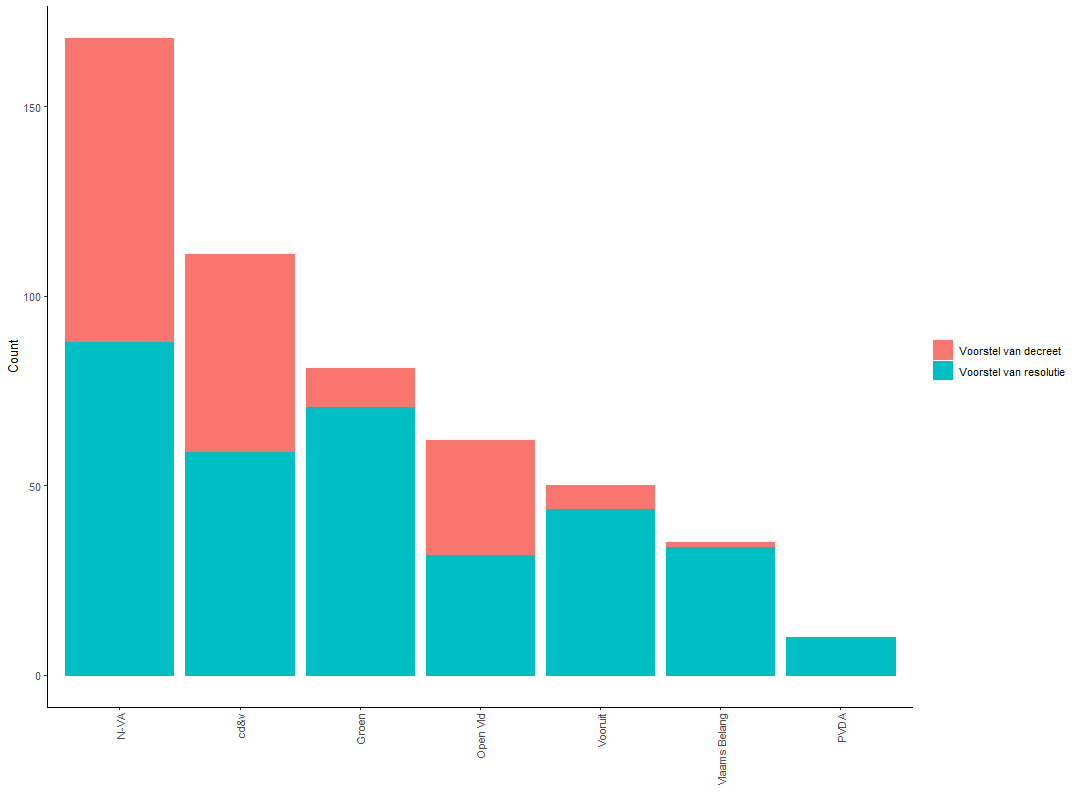
Now we can make a count of the observations by relevant types of activity and party or visualize the results. First, we filter out legislative proposals made by MPs (‘Voorstel van decreet’) and resolutions (‘Voorstel van resolutie’).

pi_type_party %>%
  filter(result_objecttype_naam == "Voorstel van decreet" 
         | result_objecttype_naam == "Voorstel van resolutie") -> pi_type_party_c

Next, we group our data by party to arrive at a count. Alternatively, we can plot the results.

pi_type_party_c %>% 
  group_by(result_contacttype_contact_fractie_naam) %>%
  count(result_objecttype_naam, sort = T) -> pi_type_party_cc

plot6 <- ggplot(pi_type_party_cc, aes(x = reorder(result_contacttype_contact_fractie_naam, -n), y = n, fill = result_objecttype_naam, colour = result_objecttype_naam)) + 
  geom_bar(stat ="identity") +
  labs(x="", y = "Count") + 
  theme_classic() +
  theme(axis.text.x = element_text(angle = 90, vjust=.5, hjust=1)) +
  theme(legend.title = element_blank())
plot6  

3. Voting records: Unnesting of the column result_journaallijn-stemmingen

pi_work %>%
  select(id_fact, 'result_journaallijn-stemmingen', result_objecttype) %>%
  unnest_wider(result_objecttype, names_sep = "_") %>%
  unnest_wider('result_journaallijn-stemmingen') %>%
  unnest_longer(stemming) %>%
  unnest_wider(stemming) -> votes

One potential observation we can make is whether the MPs of opposition parties vote against ‘ontwerp van decreet’ (i.e. those legislative proposals stemming from the Flemish government) and whether the MPs of the governing parties systematically vote in favor? Even more unnesting is needed for this, specifically of the columns stemming-tegen, stemming-voor and fractie. We start we the votes against.

votes %>%
  unnest('stemming-tegen', names_sep = "_") %>%
  unnest_wider('stemming-tegen', names_sep = "_") %>%
  unnest_longer('stemming-tegen_persoon') %>%
  unnest_wider('stemming-tegen_persoon')  %>%
  unnest(fractie, names_sep = "_") -> votes_against

We can then assess the average percentage of MPs per party voting against legislative proposals initiated by the government.

votes_against %>%
  select(id_fact, fractie_naam, `fractie_zetel-aantal`, result_objecttype_naam) %>%
  group_by(id_fact) %>%
  filter(result_objecttype_naam == "Ontwerp van decreet") %>% 
  add_count(fractie_naam) %>% 
  rename("votes_against" = "n") -> votes_against2

votes_against2 <- unique(votes_against2) 
votes_against2 <- na.omit(votes_against2) 

Same procedure for the votes in favor. First, unnesting the relevant columns.

votes %>%
  unnest('stemming-voor', names_sep = "_") %>%
  unnest_wider('stemming-voor', names_sep = "_") %>%
  unnest_longer('stemming-voor_persoon') %>%
  unnest_wider('stemming-voor_persoon')  %>%
  unnest(fractie, names_sep = "_") -> votes_infavor

We can then assess the average percentage of MPs per party voting in favor of legislative proposals initiated by the government.

votes_infavor %>%
  select(id_fact, fractie_naam, `fractie_zetel-aantal`, result_objecttype_naam) %>%
  group_by(id_fact) %>%
  filter(result_objecttype_naam == "Ontwerp van decreet") %>% 
  add_count(fractie_naam) %>% 
  rename("votes_favor" = "n") -> votes_infavor2

votes_infavor2 <- unique(votes_infavor2) 
votes_infavor2 <- na.omit(votes_infavor2) 

Next, we join the data frames to assess the voting patterns of governing and oppositions parties regarding the legislative proposals initiated by government.

votes_records <- full_join(votes_against2, votes_infavor2, by=c("id_fact" = "id_fact", "fractie_naam" = "fractie_naam", "fractie_zetel-aantal" = "fractie_zetel-aantal", "result_objecttype_naam" = "result_objecttype_naam")) 

votes_records %>% 
  mutate(votes_favor = replace_na(votes_favor, 0)) %>% 
  mutate(votes_against = replace_na(votes_against, 0)) -> votes_records2

Do the opposition parties mostly vote against and governing parties in favor?

votes_records2 %>%
  group_by(fractie_naam) %>%
  mutate(prop_against = votes_against/`fractie_zetel-aantal`) %>%
  summarise(m = mean(prop_against)) %>%
  rename("average prop. against" = "m", "party" = "fractie_naam" ) -> votes_records_against

votes_records2 %>%
  group_by(fractie_naam)  %>%
  mutate(prop_favor = votes_favor/`fractie_zetel-aantal`) %>%
  summarise(m = mean(prop_favor)) %>%
  rename("average prop. favor" = "m", "party" = "fractie_naam" ) -> votes_records_infavor